A support-response chart puts email ahead of chat: 75% of email requests met the target, compared with 66.7% for chat. Before using that comparison to guide a product or engineering decision, I'd want to know which requests the bars count. In this example, some requests appear twice, one disappears, and missing times become instant responses.
The records, faulty analysis and charts below are constructed teaching examples, produced offline. They are not a captured ChatGPT response or a report from a real support team. Product documentation was checked September 27, 2026.
OpenAI's data-analysis documentation describes working with uploaded files, producing tables and charts, and using Python for some analysis tasks. It recommends reviewing the generated code, outputs and assumptions. For a lead reviewing an analysis, that means asking for the intermediate tables and method behind the chart. Available features depend on the account and surface; a successful upload alone doesn't establish that the entire file was analyzed.
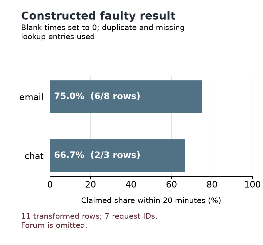
Faulty percentages from the deliberately altered data. The email bar counts eight transformed rows, although the original export has only four email requests.
Define what a row means
A CSV is a text file containing a table, with values separated by commas. Our export has one row per completed support request in a single reporting window. The question is how often each queue met a first-response target of at most 20 minutes.
| Request ID | Queue code | Recorded response minutes |
|---|---|---|
| R01 | 0 | |
| R02 | 10 | |
| R03 | 25 | |
| R04 | blank | |
| R05 | chat | 5 |
| R06 | chat | 20 |
| R07 | chat | 30 |
| R08 | forum | blank |
Zero is a recorded immediate response. A blank means the measurement is unknown. It tells us neither that a response took zero minutes nor that it was late. Exactly 20 minutes meets the target.
Those definitions let us check the result by hand. R01, R02, R05 and R06 are confirmed within target. R03 and R07 are late. R04 and R08 remain unknown. The unit we intend to count is a request, identified by its ID.
In a real export, I'd establish that unit before asking for a percentage. A row might instead represent a message, a status change or one of several attempts on the same request. Counting those rows would answer a different question.
The downloadable exercise includes both source CSVs, full Python code, the chart data and the figures. You can follow the eight records here without running it, or reproduce the calculations from the extracted files.
Follow the requests through the join
A second table supplies readable queue names. Adding those names by matching queue codes is a join. The queue code is the lookup key.
| Queue code | Queue name |
|---|---|
| Email support | |
| Email support | |
| chat | Live chat |
Email appears twice. Forum has no entry. Neither problem is visible in a finished bar labeled “Email support.”
A left join keeps unmatched requests, but each matching lookup row produces a match. With this lookup, R01 appears twice, as do the other three email requests. The result has 12 rows representing eight IDs. A percentage calculated from those rows gives email requests extra weight in a combined result, even if the duplicate labels happen to agree.
An inner join retains only requests with a matching label. To isolate that effect, use a control lookup with one email entry and one chat entry. The result has seven rows: R08, the forum request, has disappeared. It is still part of the reporting population.
The faulty chart combines an inner join against the original duplicated lookup with another error: replacing blank times with zero. It has 11 rows but only seven request IDs. R04 appears twice with an invented zero-minute time; R08 vanishes. Its chart input is:
| Queue | Transformed rows | Apparent within-target rows | Plotted percentage |
|---|---|---|---|
| 8 | 6 | 75.0% | |
| chat | 3 | 2 | 66.7% |
Across that altered table, eight of 11 rows appear within target. Neither that fraction nor the email bar describes the original requests faithfully.
I'd ask for the IDs and their occurrence counts before and after the join. A total row count is useful, but an eight-row result can still be wrong: remove R08 and add a second R01, and the count stays eight. Comparing ID multiplicities exposes both changes.
For this exercise, the raw queue codes are sufficient to calculate the valid summary. I'd retain them and report the duplicate email key and missing forum mapping. For a real lookup, the owner of the mapping needs to establish the correction. Silently taking the first match conceals that decision.
State the denominator
The denominator is the population counted in the bottom half of a fraction. Here, four of eight requests are confirmed within target: 50%. Two are late, and two lack a recorded time. Calling 50% the actual within-target rate would treat both unknowns as failures without evidence.
Among requests with recorded times, four of six are within target: 66.7%. That calculation is valid. Its label must say that it covers recorded times. It cannot establish the rate for all eight requests unless the missing measurements are resolved or additional assumptions are justified.
Replacing blanks with zero produces six apparent successes out of eight. That operation changes the data's meaning. Zero was already a valid measurement for R01; reusing it as a substitute for “unknown” makes the invented responses indistinguishable from the recorded immediate one.
The actual all-request share could be as low as four of eight if both unknowns were late, or as high as six of eight if both were within target. Those are arithmetic possibilities, not confidence intervals. This exercise makes no inference from the eight requests to a larger population.
Draw the quantities the data establish
I'd give the reader counts with unknown measurements still visible:
| Queue | All requests | Confirmed within target | Late | Unknown |
|---|---|---|---|---|
| 4 | 2 | 1 | 1 | |
| chat | 3 | 2 | 1 | 0 |
| forum | 1 | 0 | 0 | 1 |
| All | 8 | 4 | 2 | 2 |
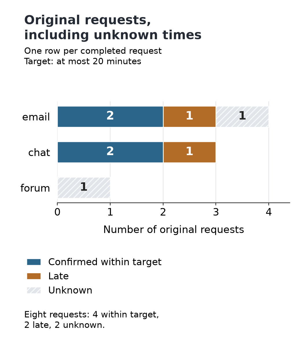
Corrected counts from the original records. The horizontal axis counts requests; unlike the first chart, it does not plot percentages. Numeric labels and the table preserve the information without relying on color.
The queue comparison now has a condition the first chart hid. Chat has two of three requests within target. Email has two of four confirmed, with one unknown: its actual within-target share could be 50% or 75%. Depending on that missing time, email could fall below or above chat. Forum's sole measurement is unknown, so zero confirmed successes does not establish zero actual successes.
Even the valid recorded-time statistic has a useful limit. Email and chat each have two of three recorded times within target. Forum has no recorded times, so that rate is undefined for forum. Reporting it as zero would invent a denominator with observations in it.
Ask for a result you can use
For this dataset, I'd request a revised analysis in these terms:
Keep one occurrence of each original request ID and retain all three raw queue codes. Treat blank times as unknown and include exactly 20 minutes within target. Show confirmed-within, late and unknown counts, then label each percentage with its numerator and denominator. Report the duplicate and unmatched lookup keys. Supply the transformation code and the exact table plotted by each chart.
In a real analysis, retain the input export, its reporting window and the resulting code and tables. OpenAI's file-review guidance recommends identifying the expected structure and review criteria, inspecting the output, and requesting focused revisions. A generated explanation is useful context; the records and calculations still have to agree.
Before acting on a queue ranking, I’d resolve the missing times and lookup labels, then recompute the comparison from the original request IDs.